
Insights from Wardriving Data
- 12 minsIntroduction
The dataset I chose for this post is one I personally collected during wireless surveys conducted around the Syracuse University campus. Otherwise known as wardriving, using the aircrack-ng suite of software I collected data about the various local wlan environments including BSSID, SSID, security type, devices connected, and signal strength at multiple locations surrounding campus. Like much hacker software, the tools used for the survey were open source with varying driver support, as a consequence of the spotty support strange results and other issues are prevalent in the data. For this project I hope to first import and clean the data which should be a difficult task given the various nulls and inconsistent format. With a clean dataframe I would like to conduct some simply analysis.
Import Data
The code below should list all the files in our /data directory and then read them into a series of dataframes.
# we need the os package to get files in directory
import os
import pandas as pd
import numpy as np

# Get a list of data_files in the data folder
dir_list = os.listdir("data/")

# .DS_Store is a hidden file found in directories on the macOS operating system
dir_list.remove(".DS_Store")
# Now we should iterate through the list and open each data_file to a dataframe
frame_list = []

for f_name in dir_list:
    df = pd.read_csv('data/'+f_name,index_col=False, header=0,error_bad_lines=False)
    frame_list.append(df)
b'Skipping line 109: expected 15 fields, saw 16\n'
Concatenate and Clean Data
For this part I will first add a new column to each of the data frames with its specific index in the list. This index is also indicative of the location where the data was collected. This will be a useful value to bin our data on and be used in the later analysis. In addition to adding some variables I conducted some mean subsitution where necessary and check data types.
# Before we are going to concatenate all of the
#  dataframes together we want to add a label so we
#  know what site they came frome
for frame_index,dframe in enumerate(frame_list):
    dframe['Location'] = frame_index
# Now I creat my big data frame putting the locations together
# so I can do some analysis and more cleaning
my_data = pd.concat(frame_list, axis=0, ignore_index=True, sort=False)
Description / Analysis
Summary Analysis
Using the describe() method of a pandas dataframe yields several very interesting and insightful statistics about the wardriving data. Some points of interest I found for the non numeric variables I outlined below:
-
Channel: 66 different unique wifi channels (frequency) with the most popular being channel 11 on 2.4ghz
-
Manufacturer: 19 Different wifi manufacturers, not as many as I would have thought but consider the few options a place like best buy offers for home routers. Manufacturers were determined by MAC address
-
Privacy: This is what many wardrivers are interested in, we can see the prevalence of WPA2 which is good, it means most people are securing their networks with the latest security.
-
Authentication: Related to privacy this is the type of auth used to access the network, most common is PSK or Pre shared key, this is the most common setup in a home network in which all users access the network with the same password.
Numeric variables describe also yielded some interesting insight:
-
Power: usually measured as dBm the power of the signal recieved, the average of the signal strength can give us an idea for how powerful the average AP’s antenna’s are. With the mean at -73.45 dBm and an IQR of ~13.00 it is apparent that most access points are at about the same power which makes sense given they all must adhere to the FCC rules governing transmit power.
-
ID-length: the length of characters in a given wifi networks name. This is very intersting because we can see the average length of a network name as well as the maximum and minimum. The mean length of a network name is 11.6 characters with a maximum length of 32 characters and a minimum or 0 (hidden network).
-
Beacons: Beacons are wireless frames containing network information which are broadcasted at a certain rate to all devices in range. The number of beacons is interesting for the same reason why Power is, we can see how close the average network is and how much data on average is communicated from the AP to the wardriver. On average an AP sent over 5.505 beacons to the listener, pretty good.
my_data.describe(include="all")
| BSSID | Manufacturer | First time seen | Last time seen | channel | Speed | Privacy | Cipher | Authentication | Power | # beacons | # IV | LAN IP | ID-length | ESSID | Location | Key | |
|---|---|---|---|---|---|---|---|---|---|---|---|---|---|---|---|---|---|
| count | 956 | 208 | 956 | 956 | 956.0 | 956.0 | 956 | 904 | 894 | 894.000000 | 894.000000 | 746.000000 | 746 | 894.000000 | 894 | 956.000000 | 686 |
| unique | 931 | 19 | 249 | 232 | 66.0 | 22.0 | 35 | 14 | 3 | NaN | NaN | NaN | 1 | NaN | 543 | NaN | 2 |
| top | BA:00:C6:7F:08:DF | Cisco Systems, Inc | 2017-11-10 19:03:47 | 2017-11-10 18:13:02 | 11.0 | 54.0 | WPA2 | CCMP | PSK | NaN | NaN | NaN | 0. 0. 0. 0 | NaN | NaN | ||
| freq | 8 | 140 | 29 | 28 | 136.0 | 634.0 | 679 | 678 | 646 | NaN | NaN | NaN | 746 | NaN | 72 | NaN | 684 |
| mean | NaN | NaN | NaN | NaN | NaN | NaN | NaN | NaN | NaN | -73.456376 | 5.505593 | 1.815013 | NaN | 11.652125 | NaN | 3.689331 | NaN |
| std | NaN | NaN | NaN | NaN | NaN | NaN | NaN | NaN | NaN | 16.699766 | 9.027981 | 17.650160 | NaN | 6.527126 | NaN | 2.220026 | NaN |
| min | NaN | NaN | NaN | NaN | NaN | NaN | NaN | NaN | NaN | -91.000000 | 0.000000 | 0.000000 | NaN | 0.000000 | NaN | 0.000000 | NaN |
| 25% | NaN | NaN | NaN | NaN | NaN | NaN | NaN | NaN | NaN | -83.000000 | 1.000000 | 0.000000 | NaN | 9.000000 | NaN | 2.000000 | NaN |
| 50% | NaN | NaN | NaN | NaN | NaN | NaN | NaN | NaN | NaN | -78.500000 | 4.000000 | 0.000000 | NaN | 12.000000 | NaN | 4.000000 | NaN |
| 75% | NaN | NaN | NaN | NaN | NaN | NaN | NaN | NaN | NaN | -70.000000 | 7.000000 | 0.000000 | NaN | 14.000000 | NaN | 6.000000 | NaN |
| max | NaN | NaN | NaN | NaN | NaN | NaN | NaN | NaN | NaN | -1.000000 | 114.000000 | 332.000000 | NaN | 32.000000 | NaN | 7.000000 | NaN |
Analysis
To get some more insight into the data I wanted to create some visualizations to help understand certain questions I had in addition to some more sophisticated data wrangling.
Which Location Has the highest average transmission power?
To answer this question I have to bin the dataframe by location and calculate mean power for each location. From the table I printed below we can see that the Power level is highest in location 1 at -71.782 and lowest at location 0 with a power level of -78.933 dBm
# First create a loop to get all of the locations
power_means = []

for loc_numb in range(7):
    # select only location part of Dataframe
    new_df = my_data.loc[my_data['Location'] == loc_numb]
    # calculate mean power
    mean_power = new_df[" Power"].mean()
    # append mean power to list
    power_means.append(mean_power)
# print header
print("Location |  Power Level\n")

# Print out results and location
for loc_val,power_val in enumerate(power_means):
    print(loc_val,"       | ",power_val)
Location |  Power Level

0        |  -78.93333333333334
1        |  -71.78260869565217
2        |  -73.39189189189189
3        |  -73.27118644067797
4        |  -75.51886792452831
5        |  -71.91428571428571
6        |  -71.85185185185185
Which location has the most open/vulnerable networks?
If we pretend for a moment that we are someone with bad intentions our data analysis skills can help us to look for vulnerabilities or the best area to attack. If we are nefarious war drivers we can find which areas to hit based on who has the less secure/ unsecure networks.
Based on the table printed below we can see that zone 2 would be the best area for a hacker to setup shop if they wanted a target rich environment with multiple vulnerable networks. At 57 open networks there is no shortage of WLANs a hacker could connect to without interference in this location. The second best locations are 0 and 1 with only 17 open networks.
priv_counts = []

for loc_numb in range(7):
    # select only location part of Dataframe
    new_df = my_data.loc[my_data['Location'] == loc_numb]
    # calculate length of privacy column where value is OPN or open network!
    priv_count = len(new_df[new_df[' Privacy'] == ' OPN'])
    # append mean power to list
    priv_counts.append(priv_count)
# print header
print("Location |  OPN Count\n")

# Print out results and location
for loc_val,priv_val in enumerate(priv_counts):
    print(loc_val,"       | ",priv_val)
Location |  OPN Count

0        |  17
1        |  17
2        |  57
3        |  15
4        |  0
5        |  2
6        |  5
Visualizations
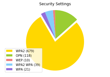
I wanted to make a pie chart to show the security features of all of the networks, This is some code I had used to initally analyze some other aspects of the data however it has been adapted here for this analysis of security types on the network.
import matplotlib.pyplot as plt

## Create labels
privlist = my_data[' Privacy'].tolist()
labels = [' WPA2',' OPN', ' WEP', ' WPA2 WPA', ' WPA']
sizes = [privlist.count(' WPA2'), privlist.count(' OPN'), privlist.count(' WEP'), privlist.count(' WPA2 WPA'), privlist.count(' WPA')]

# Draw the piechart
colors = ['gold', 'yellowgreen', 'lightcoral', 'lightskyblue','mediumpurple']
explode = (0.1, 0, 0, 0,0)  # explode 1st slice
labels2 = []
# for loop to create labels for key
for i in range(len(labels)):
    tempstr = labels[i] + " ("+str(sizes[i])+") "
    labels2.append(tempstr)


# Plot our chart
patches, texts = plt.pie(sizes, explode=explode ,colors=colors, startangle=120)
plt.legend(patches, labels2, loc="best")
plt.title('Security Settings')
plt.axis('equal')
plt.show()
Conclusion
This dataset shows how interesting insight can be derived from data that looks confusing and unstructured at first. The tremendous power of Pandas dataframes and python are evident, I’m sure some excel gurus could have done this without programming at all, but the benefits of programming are endless. Now we have a base for a small script which could do more analysis on the fly during future wardrives, automating a large part of our inital analytical process. Despite my apprehensions about working with this data I am very pleased with how everything turned out.

Nicholas L Brown
Data Scientist