
Visual Analysis of Fishing Data with Python
- 44 minsI. Overview
For this project I decided to use the scripting skills I learned to build a python program which could analyze data from my various fishing trips. By the end of this project I hope to demonstrate how I can import, analyze, and question my fishing data attempting to understand more about what makes a successful trip. This notebook was used to import, clean, and do analysis on the data. In the future I would leave the data processing up to python and move the visualization portion to a tool like Tableau or Power BI.
II. Dataset Description and Source
Data for this analysis was generated using a python coded data generator. I ended up with a small dataset of around 400 lines with 4 columns. By the end of this analysis I hope to have extended the number of variables in this catch dataset significantly and derive some actionable insight from it. The initial dataset has only four columns: species caught (the name of the fish), latitude, longitude, and datetime of the catch. Later on in part five the final three columns will be used to make various API queries to extend the dataset. Finally in part six I will be doing my final analysis seeking to tie together the data into a coherent answer to my question.
III. Dataset Pre-processing
For this part I will import and clean the original information imported into the dataset which will allow me to ask my analysis questions later in this report. Though I originally wanted to make a whole system dedicated to managing new entries I decided that I needed more data to get the application framework started else both myself and the program would lack any data to actually conduct analysis on. For this part I worked in multiple steps:
- Import dataset
- Quick analysis of missing values etc.
- Clean dataset (from my quick overview there appeared to be some null values)
Import Packages
These are the packages necessary for the pre-processing steps
import pandas as pd
import os
Read in Dataset
The dataset I want to read in is a .csv file, the variables include location (as lattitude and longitude), species (limited to three), and the datetime of the catch. We will end this section with a dataframe called catchesDF
# Get a list of data_files in the data folder
dir_list = os.listdir("data/")

# .DS_Store is a hidden file found in directories on the macOS
#  -operating system
if '.DS_Store' in dir_list:
    dir_list.remove(".DS_Store")
# Import catches csv
catchesDF = pd.read_csv('data/'+dir_list[0],index_col=False
                         , header=0,error_bad_lines=False)

locationDF = pd.read_csv('data/'+dir_list[1],index_col=False
                         , header=0,error_bad_lines=False)
# Make sure catch data is imported
catchesDF.head(5)
| Species Caught | Latitude | Longitude | Datetime | |
|---|---|---|---|---|
| 0 | Striped Bass | 41.179744 | -72.047878 | Mon, 18 Jun 2018 06:37 -0500 |
| 1 | Striped Bass | 41.084336 | -71.945062 | Tue, 4 Jul 2017 12:15 -0500 |
| 2 | Striped Bass | 41.084485 | -72.007186 | Tue, 20 Nov 2018 05:06 -0500 |
| 3 | Striped Bass | 41.078046 | -71.978532 | Wed, 6 Feb 2019 04:39 -0500 |
| 4 | Striped Bass | 41.150089 | -71.994974 | Thu, 1 Mar 2018 08:50 -0500 |
locationDF.head(5)
| Location Name | Latitude | Longitude | Target | |
|---|---|---|---|---|
| 0 | Montauk Point (The Elbow) | 41.070783 | -71.854206 | Striped Bass, Black Seabass, Bluefish |
| 1 | Blackfish Rock | 41.079974 | -71.882730 | Striped Bass, Blackfish |
| 2 | Ditch Plains | 41.038796 | -71.916757 | Striped Bass |
| 3 | Fort Tyler (The Ruins) | 41.141555 | -72.145713 | Striped Bass, Fluke, Bluefish |
| 4 | Plum Gut | 41.165869 | -72.215735 | Striped Bass |
Clean Dataset
In this part I wanted to clean up the data and decide what to do with certain null values. Because I wanted to get as much data as possible I was willing to take coordinates and datetimes without knowing the target species. In this part I will clean up the catchesDF and assign the null values based on my domain knowledge.
# First, I will look if there are any nulls present in the dataset
catchesDF.isnull().sum()
Species Caught    15
Latitude           0
Longitude          0
Datetime           0
dtype: int64
Replace Null Values
Based on the output above we can see that around 15 entries are missing a species name. For this analysis I would like to replace them with the species name ‘Striped Bass’ because that is by far the most common in the dataset. Below is some code which will do that.
# Replace all NA's in the 'species caught' column with striped bass
# - this function returns a new dataframe so lets reassign the old one
catchesDF = catchesDF.fillna({"Species Caught":"Striped Bass"})
# Now lets make sure it worked
catchesDF.isnull().sum()
Species Caught    0
Latitude          0
Longitude         0
Datetime          0
dtype: int64
IV. Initial Dataset Exploratory Analysis
Now that we have a bare-minimum clean dataset as a starting point I want to conduct a quick analysis and exploration before we add features to better understand the dataset. Some initial exploration questions I want to answer are:
- What are the most popular species in the dataset ?
- What do each of the years of fishing look like ?
- Are there any popular coordinates for fishing so far?
Imports
These are the packages necessary for our exploratory analysis
import matplotlib.pyplot as plt
import numpy as np
from mpl_toolkits.basemap import Basemap
Which Species are Most Popular?
I find visual aids to be very effective for exploratory analysis so I hope to use both numbers and visuals to answer the questions above starting with getting an idea of what species the people who helped me collect this data are targeting. From my extensive time spent collecting the data I know that it will most likely be the striped bass but a chart will help to show the exact disparity between the two.
specDF = catchesDF.groupby('Species Caught').count()[['Datetime']]
specDF = specDF.rename(columns = {"Datetime":"Count"})
#specDF = specDF.reset_index()
specDF
| Count | |
|---|---|
| Species Caught | |
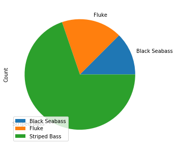
| Black Seabass | 50 |
| Fluke | 71 |
| Striped Bass | 279 |
Analysis of Species Question - Pie Chart
From the dataframe above we can see that Striped Bass make up more than 50% of the dataframe. Lets see what a piechart may look like so we can see just how much of the data is striped bass fishing
specDF.plot(kind='pie', subplots=True, figsize=(5, 5))
plt.subplots_adjust(right=20)
plt.show()
How Good Was the Fishing During Various Years?
For this part I just want to get an idea of what dates have the highest counts where fish were caught. This part required some tricky code as I have to deal with datetime objects. I found a quick and pretty sloppy way of doing it but it worked much easier and faster than creating datetime objects in python.
yearlist = []

# This for loop will create a list of the various years present in the dataset
for index, row in catchesDF.iterrows():
    if '2017' in row['Datetime']:
        yearlist.append('2017')
    elif '2018' in row['Datetime']:
        yearlist.append('2018')
    elif '2019' in row['Datetime']:
        yearlist.append('2019')

catchesDF["year"] = yearlist
yearDF = catchesDF.groupby('year').count()[['Datetime']]
yearDF = yearDF.rename(columns = {"Datetime":"Count"})
Analysis of Dates Question - Histogram
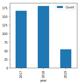
The histogram can help to visualize the number of fish caught per year in the dataset. We can see that 2017 and 2018 were good years. Given that it is only the beginning half of 2019 this is actually a very interesting chart. This chart helps to show how the summer months are where the real catch productivity is. We will look at the dates in a more granular fashion later but for now this is an interesting description of the initial dataset.
yearDF.plot(kind="bar", figsize = (4,4))
plt.show()
Where is Most of the Fishing Happening?
This part was the most complicated but I also felt it would be the most rewarding. Below is the code necessary to create a visualization of all of the latitude and longitude points present in the initial dataset. Becase there are some 400 points I assume this will end up looking like a scatterplot with a map as the background. I hope this will allow me to identify some clusters of fishing areas. Because of the way the package ‘basemap’ works I had to use some clever scripting and python skills I learned to give basemap a square coordinates system.
# Get min and max of longitude and latitude
latmax = catchesDF["Latitude"].max()
latmin = catchesDF["Latitude"].min()

lonmax = catchesDF["Longitude"].max()
lonmin = catchesDF["Longitude"].min()

# get lats and lons as list, we'll use these later for our map
lats = catchesDF['Latitude'].tolist()
lons = catchesDF['Longitude'].tolist()
# These coordinates should give us the area which contains all the points
# -If I put them in correctly below they should focus our map on the
# -fishing grounds

print(latmax,latmin,lonmax,lonmin)

print(lats[:4],lons[:4])
41.20673767 41.01277836 -71.78484526 -72.37182677
[41.17974427, 41.08433606, 41.08448546, 41.07804553] [-72.04787783, -71.94506225, -72.00718632, -71.97853245]
Analysis of Location Question - Map
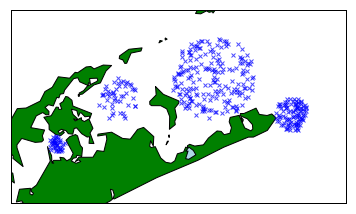
Below is the code which actually draws our map. Because the area is local to me I recognize it however I could see that if you arent familiar with the area the map doesn mean a whole lot. Regardless of context this map yielded some very interesting and useful results. We can see now that there are 4 major fishing clusters some more dense than others. Later on we will see how my fishing spot locations compare to these clusters. If we wanted we could be using that table to assign these clusters some names.
map = Basemap(projection='merc',
    resolution = 'h', area_thresh = 10,
    llcrnrlon=lonmin-.09, llcrnrlat=latmin-.09,
    urcrnrlon=lonmax+.09, urcrnrlat=latmax+.05)

map.drawcoastlines()
map.drawcountries()
map.fillcontinents(color = 'green', lake_color = "lightblue")
map.drawmapboundary()
x,y = map(lons,lats)
map.plot(x,y,'bx',markersize=4, alpha = .7)
map.drawlsmask(ocean_color = 'lightblue')
plt.show()
V. Dataset Build Out
This part of the assignment I will be using APIs to build out the dataset obtaining some new information. After this process is complete we will have a dataset where some serious analysis can be done combining the lookup data with our current dataset. Because we have a date/time and location (Latitude and Longitude) we can easily get other information derived from these few data points. This is great because we dont have to worry about maintaining an entire database with tides, weather, and other information which there are entire organizations dedicated to collecting. Though we may want to store our heavily modified dataframe later to avoid excessive lookups and queries.
Imports
These are the packages necessart for the dataset build out portion
from datetime import datetime
import requests
import json
import time
Use NOAA API to add Water Temp to Dataframe
As a first addition to the catches dataframe I will be using the NOAA API and library ‘requests’ to simply request the current water temperature at each of the locations and times of catches. I will eventually need to think of a solution for mapping these to lat/lon or the software will be un-usable outside the eastern long island area. I suspect the largest challenge for this part will be formatting the dates.
# station ID which is nearest to the fishing grounds
station_id = '8510560'

# Water Temp List
water_temps = []

# URL for API
url = 'http://tidesandcurrents.noaa.gov/api/datagetter?'

# for loop to loop through dataframe
for index, row in catchesDF.iterrows():

    # need to convert string to datetime_object ex. (Fri, 6 Jun 2018 17:18:56 -0500)
    try:
        datetime_object = datetime.strptime(row['Datetime'], '%a, %d %b %Y %H:%M %z')
    except:
        datetime_object = datetime.strptime(row['Datetime'], '%a, %d %b %Y %H:%M:%S %z')
    date_to_send = datetime_object.strftime('%Y%m%d')
    #print(date_to_send)

    # Assemble payload
    payload = {'station': station_id, 'end_date': date_to_send,
               'range': '24', 'product':'water_temperature','format':'json',
                'units':'english', 'time_zone':'lst'}

    data = requests.get(url, params=payload)
    json_data = json.loads(data.text)

    try:
        water_temps.append(float(json_data['data'][0]['v']))
        #print("Got temp for :",row['Datetime'])
    except:
        water_temps.append(np.NaN)
        #print("Could not get temp for :",row['Datetime'])

    time.sleep(1)

# Append our list to the main data
catchesDF['Water Temp. (F)'] = water_temps
Checkout the new ‘Water Temp’ column
Below I wanna see how the code worked out. It looks like there were some null values produced from the API which isnt perfect. This is a great opportunity to do some mean substition and clean up the dataframe a bit more. It seems like only times from 2017 so lets do some mean substitution for the mean of 2017 we could collect.
# Now I will calculate the mean water temp for 2017 and see how many NaNs we have
catchesDF.isnull().sum()
Species Caught      0
Latitude            0
Longitude           0
Datetime            0
year                0
Water Temp. (F)    77
dtype: int64
mean_temp = catchesDF['Water Temp. (F)'].mean()
catchesDF = catchesDF.replace(np.NaN,mean_temp)
# Make sure our mean substitution worked
catchesDF.isnull().sum()
Species Caught     0
Latitude           0
Longitude          0
Datetime           0
year               0
Water Temp. (F)    0
dtype: int64
catchesDF.head(5)
| Species Caught | Latitude | Longitude | Datetime | year | Water Temp. (F) | |
|---|---|---|---|---|---|---|
| 0 | Striped Bass | 41.179744 | -72.047878 | Mon, 18 Jun 2018 06:37 -0500 | 2018 | 64.0 |
| 1 | Striped Bass | 41.084336 | -71.945062 | Tue, 4 Jul 2017 12:15 -0500 | 2017 | 71.4 |
| 2 | Striped Bass | 41.084485 | -72.007186 | Tue, 20 Nov 2018 05:06 -0500 | 2018 | 51.6 |
| 3 | Striped Bass | 41.078046 | -71.978532 | Wed, 6 Feb 2019 04:39 -0500 | 2019 | 37.4 |
| 4 | Striped Bass | 41.150089 | -71.994974 | Thu, 1 Mar 2018 08:50 -0500 | 2018 | 40.6 |
Use NOAA API to Add Other Features to Dataset
Now that we can see our water temp worked out lets try out getting other variables like pressure and wind direction from the same NOAA API. Again I anticipate some issues which we can work out with mean substitution. This time I will create multiple payloads to send to the server which should query all the columns we want. I have chose 4 more columns to add based on what was available form the API:
- Wind Speed (MPH)
- Wind Direction
- Air Temperature (F)
- Air Pressure (mbar)
Add Air Temperature (in Degrees Fahrenheit)
This one is most similar to the water temp API call so I decided to start with this.
# Air Temp List
air_temps = []

# for loop to loop through dataframe
for index, row in catchesDF.iterrows():

    # need to convert string to datetime_object ex. (Fri, 6 Jun 2018 17:18:56 -0500)
    try:
        datetime_object = datetime.strptime(row['Datetime'], '%a, %d %b %Y %H:%M %z')
    except:
        datetime_object = datetime.strptime(row['Datetime'], '%a, %d %b %Y %H:%M:%S %z')
    date_to_send = datetime_object.strftime('%Y%m%d')
    # Assemble various payloads (One for )
    payload = {'station': station_id, 'end_date': date_to_send,
               'range': '24', 'product':'air_temperature','format':'json',
                'units':'english', 'time_zone':'lst'}

    data = requests.get(url, params=payload)
    json_data = json.loads(data.text)
    try:
        air_temps.append(float(json_data['data'][0]['v']))
    except:
        air_temps.append(np.NaN)

# Append our list to the main dataframe
catchesDF['Air Temp. (F)'] = air_temps
mean_air_temp = catchesDF['Air Temp. (F)'].mean()
catchesDF = catchesDF.replace(np.NaN,mean_air_temp)
catchesDF.head(5)
| Species Caught | Latitude | Longitude | Datetime | year | Water Temp. (F) | Air Temp. (F) | |
|---|---|---|---|---|---|---|---|
| 0 | Striped Bass | 41.179744 | -72.047878 | Mon, 18 Jun 2018 06:37 -0500 | 2018 | 64.0 | 66.0 |
| 1 | Striped Bass | 41.084336 | -71.945062 | Tue, 4 Jul 2017 12:15 -0500 | 2017 | 71.4 | 71.8 |
| 2 | Striped Bass | 41.084485 | -72.007186 | Tue, 20 Nov 2018 05:06 -0500 | 2018 | 51.6 | 46.8 |
| 3 | Striped Bass | 41.078046 | -71.978532 | Wed, 6 Feb 2019 04:39 -0500 | 2019 | 37.4 | 40.3 |
| 4 | Striped Bass | 41.150089 | -71.994974 | Thu, 1 Mar 2018 08:50 -0500 | 2018 | 40.6 | 48.0 |
Add Air/Barometric Pressure (in millibar)
This will query the API and add air pressure in millibar. For reference one atm (atmosphere of pressure) is defined as 1013.25 mbar.
# Pressure Temp List
pressure_list = []

# for loop to loop through dataframe
for index, row in catchesDF.iterrows():
    # need to convert string to datetime_object ex. (Fri, 6 Jun 2018 17:18:56 -0500)
    try:
        datetime_object = datetime.strptime(row['Datetime'], '%a, %d %b %Y %H:%M %z')
    except:
        datetime_object = datetime.strptime(row['Datetime'], '%a, %d %b %Y %H:%M:%S %z')
    date_to_send = datetime_object.strftime('%Y%m%d')
    # Assemble various payloads
    payload = {'station': station_id, 'end_date': date_to_send,
               'range': '24', 'product':'air_pressure','format':'json',
                'units':'english', 'time_zone':'lst'}

    data = requests.get(url, params=payload)
    json_data = json.loads(data.text)
    try:
        pressure_list.append(float(json_data['data'][0]['v']))
    except:
        pressure_list.append(np.NaN)

catchesDF['Pressure (mbar)'] = pressure_list
mean_pressure = catchesDF['Pressure (mbar)'].mean()
catchesDF = catchesDF.replace(np.NaN,mean_pressure)
catchesDF.head(5)
| Species Caught | Latitude | Longitude | Datetime | year | Water Temp. (F) | Air Temp. (F) | Pressure (mbar) | |
|---|---|---|---|---|---|---|---|---|
| 0 | Striped Bass | 41.179744 | -72.047878 | Mon, 18 Jun 2018 06:37 -0500 | 2018 | 64.0 | 66.0 | 1018.6 |
| 1 | Striped Bass | 41.084336 | -71.945062 | Tue, 4 Jul 2017 12:15 -0500 | 2017 | 71.4 | 71.8 | 1016.1 |
| 2 | Striped Bass | 41.084485 | -72.007186 | Tue, 20 Nov 2018 05:06 -0500 | 2018 | 51.6 | 46.8 | 1013.8 |
| 3 | Striped Bass | 41.078046 | -71.978532 | Wed, 6 Feb 2019 04:39 -0500 | 2019 | 37.4 | 40.3 | 1019.0 |
| 4 | Striped Bass | 41.150089 | -71.994974 | Thu, 1 Mar 2018 08:50 -0500 | 2018 | 40.6 | 48.0 | 1011.3 |
Add Wind Speed and Wind Direction (in MPH)
There is a simple wind parameter we can pass to the api which will return a JSON object containing both pieces of information we want.
# Wind Lists
direction_list = []
speed_list = []
#new station id
station_id = '8461490'

# for loop to loop through dataframe
for index, row in catchesDF.iterrows():
    # need to convert string to datetime_object ex. (Fri, 6 Jun 2018 17:18:56 -0500)
    try:
        datetime_object = datetime.strptime(row['Datetime'], '%a, %d %b %Y %H:%M %z')
    except:
        datetime_object = datetime.strptime(row['Datetime'], '%a, %d %b %Y %H:%M:%S %z')
    date_to_send = datetime_object.strftime('%Y%m%d')
    #print(date_to_send)
    # Assemble various payloads
    payload = {'station': station_id, 'end_date': date_to_send,
               'range': '24', 'product':'wind','format':'json',
                'units':'english', 'time_zone':'lst'}

    data = requests.get(url, params=payload)
    json_data = json.loads(data.text)
    # Append direction list
    try:
        direction_list.append(json_data['data'][0]['dr'])
    except:
        direction_list.append(np.NaN)
    # Append speed list
    try:
        speed_list.append(float(json_data['data'][0]['s']))
    except:
        speed_list.append(np.NaN)
    #time.sleep(1)

# Append our list to the main dataframe
catchesDF['Wind Direction'] = direction_list
catchesDF['Wind Speed (MPH)'] = speed_list
mean_speed = catchesDF['Wind Speed (MPH)'].mean()
catchesDF['Wind Speed (MPH)'] = catchesDF['Wind Speed (MPH)'].replace(np.NaN, mean_speed)
catchesDF['Wind Direction'] = catchesDF['Wind Direction'].replace("", 'N')
Check out the New Dataframe
Now that we are done with our API calls we can check out our completed dataframe and also save it as a new CSV so that we dont have to make all those API queries again. First we will make sure there are no nulls left. Then we will export the dataframe as a csv file.
catchesDF.isnull().sum()
Species Caught      0
Latitude            0
Longitude           0
Datetime            0
year                0
Water Temp. (F)     0
Air Temp. (F)       0
Pressure (mbar)     0
Wind Direction      0
Wind Speed (MPH)    0
dtype: int64
catchesDF.head(5)
| Species Caught | Latitude | Longitude | Datetime | year | Water Temp. (F) | Air Temp. (F) | Pressure (mbar) | Wind Direction | Wind Speed (MPH) | |
|---|---|---|---|---|---|---|---|---|---|---|
| 0 | Striped Bass | 41.179744 | -72.047878 | Mon, 18 Jun 2018 06:37 -0500 | 2018 | 64.0 | 66.0 | 1018.6 | S | 2.53 |
| 1 | Striped Bass | 41.084336 | -71.945062 | Tue, 4 Jul 2017 12:15 -0500 | 2017 | 71.4 | 71.8 | 1016.1 | N | 2.92 |
| 2 | Striped Bass | 41.084485 | -72.007186 | Tue, 20 Nov 2018 05:06 -0500 | 2018 | 51.6 | 46.8 | 1013.8 | NNE | 1.36 |
| 3 | Striped Bass | 41.078046 | -71.978532 | Wed, 6 Feb 2019 04:39 -0500 | 2019 | 37.4 | 40.3 | 1019.0 | NNW | 10.30 |
| 4 | Striped Bass | 41.150089 | -71.994974 | Thu, 1 Mar 2018 08:50 -0500 | 2018 | 40.6 | 48.0 | 1011.3 | SSW | 0.78 |
Write Out the New Dataframe to a CSV file
catchesDF.to_csv(r'data\extended_data.csv')
VI. Main Analysis
Now that we have a dataset with way more indicators which I believe will help build a profile of successful catches helping me on my future trips. I plan on looking at each of the added indicators seperatley as well as together and in the end draw conclusions about the ideal values to look for when planning a trip. This is the part where I will answer my main question of “What are the ideal conditions for catching a fish?” in other words “What makes a successful fishing trip?”
What are the Ideal Wind Conditions?
First we will try to determine some ideal wind conditions which we can add to our successful trip profile. I think the easiest way to analyze this would be through creating a histogram and looking at the frequency of fish caught given the wind direction. Later on in the analysis a boxplot of the windspeed should help us to determine if wind factors other than direction have any effect on the fishing trip success. For now I wanted to examine the effect wind direction had on the catch species.
directionDF = catchesDF.groupby(['Wind Direction','Species Caught']).count()[['Datetime']]
directionDF = directionDF.sort_values(by=['Datetime'])
directionDF[['Datetime']].plot(kind="barh", figsize = (8,12), stacked = True, fontsize = 12)
plt.show()
Wind Direction Interpretation
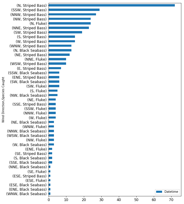
The barchart I plotted above is an excellent resource for starting to understand the particular wind conditions necessary for a successful fishing trip. I decided to subset the data by wind direction as well as species in an attempt to uncover if there are any specific trends related to both (for example, I wanted to know if the wind is blowing North should I bother with Fluke fishing or should I go for something else?). Based on the chart above we can see that Northern winds are the most successful for fishing all types of species in the dataset. We can also see that Eastern winds are the worst for any type of fishing, based on my domain knowledge this is for a few reasons: Firstly, Eastern winds create the roughest conditions on the East coast as wind blowing accross the Atlantic causes massive surf. Secondly, Eastern winds and the surf it develops bring in debris from the ocean which cause fish to move to deeper, calmer water further away from the fishing grounds.
What are the Ideal Temperature Conditions?
For this part I wanted to get an idea of which temperature conditions are most productive for fishing. I realize that fishing may pick up in the summer so warmer temps would be more popular but the dataset I collected has year round dates so I think the analysis is worthy and if interpreted properly could yield some great insight. The best way to look at this data I feel is to visualize it in a scatter plot. As with the above plot I also want to add another dimension by factorizing the fish species and coloring their points respectivley to see the range that different fish are caught in.
tempDF = catchesDF.copy()
tempDF['codes'] = tempDF['Species Caught'].astype('category').cat.codes
ax2 = tempDF.plot.scatter(x='Water Temp. (F)', y='Air Temp. (F)',figsize = (8,6),
                          c='codes', colormap='brg',s=50, alpha = .5,
                          title = "Plot of Air Temp vs Water Temp (2 = Striped Bass, 1 = Fluke, 0= Black Seabass)\n",
                         grid = True)
ax2.xaxis.tick_top()
#plt.tight_layout()
plt.show()
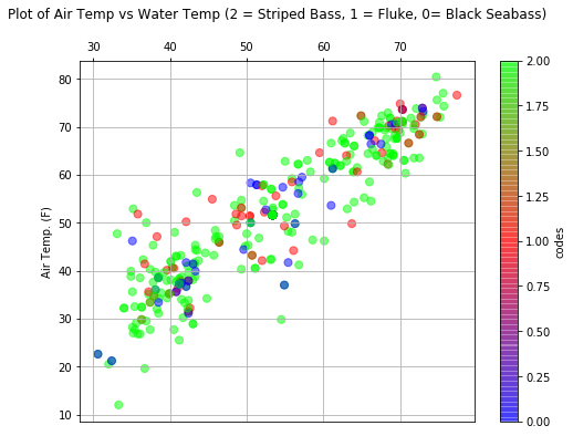
Temperature Analysis Interpretation
This scatterplot above yields some very interesting results which I think are worth going over and including in this report. First thing to note is the obvious and anticipated correlation between air temp and water temp. To cover some not so obvious interpretations let’s first look at the striped bass points (number 2 or the green points). Striped bass are the most populous species in the dataset so it makes sense to see a majority of green points on the plot. However, we can begin to identify the temperature range that the bass (and other fish) are caught in. The largest takeaway for me was the existance of two clusters where a lot of bass seemed to be caught. The first cluster exists around 40 degrees water temp and around 35 to 40 in air temp. This to me seems to be the fall blitz which usually occurs as the water rapidly cools during the months of september - december. Interestingly once the air gets below the 30s signalling winter there is very few fish caught (I suspect this is also because people want to go less once it gets very cold). The second cluster I could identify was the early summer cluster where the air temp is between 60 and 75 degrees and the water temp is between 60 and 70 degrees. This would explain why my prefered late summer fishing time is so unsuccessful, it is simply too hot for the fish. Finally I can begin to identify a cluster in between these two where Fluke fishing seems to be more successful. There is a nice grouping of red dots right around the 50 degree air temperature and 50 degree water temperature marks. Perhaps it would be a good idea to only go for the Fluke when temperatures get warmer.
How Does Barometric Pressure Influence Catches?
For this part I simply want to see the distribution of barometric pressure for the catches to better understand the ideal conditions for fishing. I often hear varying opinions on fishing before/after storms or cold/warm fronts (things indicated by barometric pressure) so it will be interesting to see what the pressure was like when most fish are caught. I think a box and whisker plot could really help to explain the data so I will check that out first. I used this article as a reference point for conventional wisdom about pressure and fish: https://weather.com/sports-recreation/fishing/news/fishing-barometer-20120328
# First lets create a seperate dataframe for our plot

boxDF = catchesDF.copy()
bplot = boxDF.boxplot(column = ['Pressure (mbar)'], by='Species Caught', figsize=(8,8))
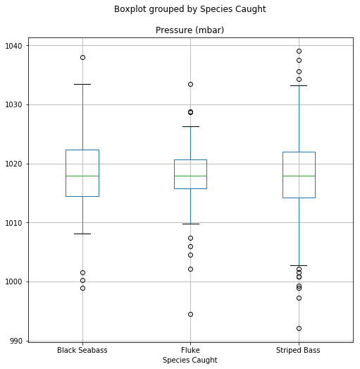
Pressure Analysis Interpretation
The first thing I noticed was the difference in pressure ranges in which the black seabass and striped bass are caught compared to the fluke. According to the article I referenced above this seems to help back up the claim made by the marine biologist that fish with larger swim bladders are more effected by atmospheric pressure prefering a higher average pressure. The Fluke (also known as Summer Flounder) is a flatfish, interestingly enough adult flatfish do not have a swim bladder as a majority of their life is spent on the sea floor. We can see comparing the fluke to both types of bass how this data completely backs up the articles assertions! Considering one atmosphere of pressure at sea level is 1013 millibar we can see the average pressure of all three species is slightly higher. The whiskers of the plot yield some great insight as well. For example we can see that the Striped Bass (the most apex predator in the list) is willing to feed in a very large range of conditions where as the black seabass much prefers the higher pressure systems. Finally we can see how fluke have a very specific range where they are usually being caught with a few outliers on either the higher or lower side. My main take away from this part is that if the pressure is high, bass fishing will be okay but flounder/fluke fishing may be off the table
How Does Wind Speed Influence Catches?
We saw above how pressure effects fishing especially considering the biology of the various species. For this part I suspect that we will see some similarities in the trends where different fish respond differently to high/low wind speeds. Before we do the analysis it’s important to understand how wind (which exists above the ocean) affects life below the surface. Wind causes waves which can determine the strength of underwater currents. Essentially if it is rough and windy on the surface, the ocean beneath will be affected similarly. That said I think that mid-water fish like both the bass species would be more okay with high winds compared to a bottom fish which could become agitated by the sand and debris being kicked up by poor weather.
# create seperate DF for analysis portion
windDF = catchesDF.copy()
bplot2 = windDF.boxplot(column = ['Wind Speed (MPH)'], by='Species Caught', figsize=(8,6), vert=False)
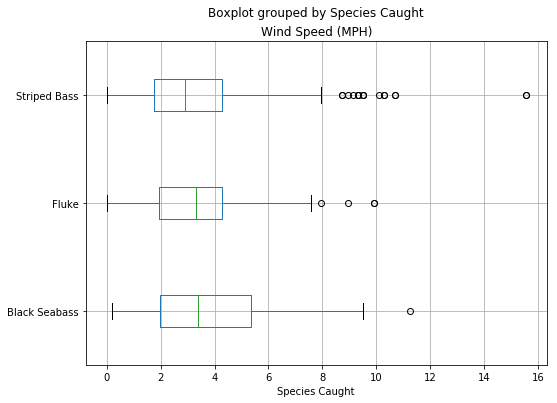
Wind Speed Analysis
The distribution of wind speed is very intersting. The first thing I noticed which was readily obvious is that rarely fish are caught when the wind is blowing over 10mph. I was pretty surprised by this until I realized that very few people would want to be out on a boat on a windy day getting rolled around by the ocean. I was very surprised to see how the black seabass could be caught in such a large range. The black seabass, compared to the fluke or striped bass, is a more of a scavenger than a predatory fish. It seems they are willing to be more active feeding on crabs or clams burried in the sand when the water is most turbulent (during windy days). Compared to the fluke or striped bass who tend to eat other fish and may be less likely to feed if their hunting ground has poor visiblity and all the smaller fish have moved out to deeper water.
What do the Current Fishing Grounds Look Like?
In this part I wanted to use the basemap package similar to the inital exploratory plot to get a map of the fishing grounds and what they might look like today. This was initally designed to be put into a flask application however I found myself doing more tinkering in javascript instead of actual analysis. It would be a great project to attempt without a hard time limit and I plan on continiung to work towards that objective. Instead of the NOAA API I will use the weather.gov API to fill out up-to-date weather information at my popular fishing locations.
tempr_list = []

# for loop to loop through dataframe
for index, row in locationDF.iterrows():
    # Define api request parameters in payload
    payload = str(row['Latitude'])[:9]+','+str(row['Longitude'])[:10]
    #print("Payload: ",payload)
    # Define URL which in our case is very simple
    url = "https://api.weather.gov/points/{0}/forecast".format(payload)
    #print("url: ",url)
    data = requests.get(url)
    json_data = json.loads(data.text)
    if 'properties' not in json_data:
        result = "API Missing Data"
        #print("Lat: ",str(row['Latitude'])[:9],"Lon: ",str(row['Longitude'])[:10], "Error Collecting Data For")
    else:
        result = json_data['properties']['periods'][0]['temperature']
    # Append temperature rsults to temp list
    tempr_list.append(result)

# Append list as column to dataframe
locationDF['Todays Temperature (F)'] = tempr_list
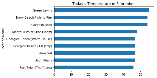
What is the Temperature at each Location Now?
Based on this information I could potentially decide where to head out when I go fishing. I will simply use the weather.gov api and return a small table containing the information.
loctempDF = locationDF[['Location Name','Todays Temperature (F)']]
loctempDF = loctempDF.set_index('Location Name')
# sort data
loctempDF = loctempDF.sort_values(by=["Todays Temperature (F)"])
# create plot
loctempDF[['Todays Temperature (F)']].plot(kind='barh',figsize = (6,4)
                                           , title = "Today's Temperature in Fahrenheit", legend = None)
plt.show()
How do the Catch Clusters Compare to the Fishing Locations?
Now we will plot both the catch clusters plotted earlier as well as the data points which are known fishing locations to determine the popularity of the various locations.
# Get min and max of longitude and latitude
latmax1 = locationDF["Latitude"].max()
latmin1 = locationDF["Latitude"].min()

lonmax1 = locationDF["Longitude"].max()
lonmin1 = locationDF["Longitude"].min()

# get lats and lons as list, we'll use these later for our map
lats1 = locationDF['Latitude'].tolist()
lons1 = locationDF['Longitude'].tolist()
map = Basemap(projection='merc',
    resolution = 'h', area_thresh = 10,
    llcrnrlon=lonmin1-.09, llcrnrlat=latmin1-.09,
    urcrnrlon=lonmax1+.09, urcrnrlat=latmax1+.05)

map.drawcoastlines()
map.drawcountries()
map.fillcontinents(color = 'green', lake_color = "lightblue")
map.drawmapboundary()
x1,y1 = map(lons1,lats1)
map.plot(x1,y1,'ro',markersize=15, alpha = 1)
x,y = map(lons,lats)
map.plot(x,y,'bx',markersize=4, alpha = .7)
map.drawlsmask(ocean_color = 'lightblue')
plt.show()
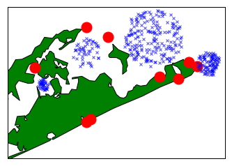
Map Analysis Interpretation
This map actually shows some potentially new great spots to try fishing! I initially thought that the catch clusters would align with my locations however this shows where the recently productive areas are. Perhaps it is time I rethought where one needs to go to catch fish especially considering the ever changing state of the ocean it is possible that patterns will become more erratic in the future and these analytical skills could help to decipher a lot of questions about the nature of the local ecosystem. For example, the largest cluster (by area) is actually east of two locations which used to be considered very popular, perhaps this shows how as summers become warmer each year the fish are moving into deeper water further away from the coast. It would also explain the very poor beach where there were no recorded catches.
VII. Conclusion
As I worked through this analysis my expectations and understanding shifted drastically. Initially I sought to produce an analysis that could tell the the optimal days and situations to fish however I soon realized that this type of analysis would not be very useful from an applied standpoint. This is because I realized most people (including myself) do not have the luxury of simply choosing the best days to fish from a list. We have jobs and family commitments which limit our fishing days to a specific window where we go regardless of specific temp/pressure (weather permitting). Realizing this I decided to move forward with a much more user centric approach whereby I sought to understand how to optomize and analyze the trips I take and the data I consume. My largest question has been answered as this analysis has helped me to understand how various metrics common on fishing reports can be interpretted.This analysis was most exciting to me because it demonstrates how someone with a little bit of data and analytical skills can gain insight and wisdom into patterns and trends previously only apparent to the most seasoned fisherman. If I want to have success I now know what locations (lat,lon) to go to when the wind is blowing North, the temperature is not too warm, and the atmospheric pressure is high.

Nicholas L Brown
Data Scientist